Spark 2.2.0: New Imputer to replace missing values

With the release of Spark 2.2.0, we can now use the newly implemented Imputer to replace missing values in our dataset. However, it only supports mean and median as the imputation strategies currently but not the most frequent. The default strategy is mean. (Note: scikit-learn provides all three different strategies).

See the Imputer class and the associated Jira ticket below
https://github.com/apache/spark/blob/master/mllib/src/main/scala/org/apache/spark/ml/feature/Imputer.scala

https://issues.apache.org/jira/browse/SPARK-13568

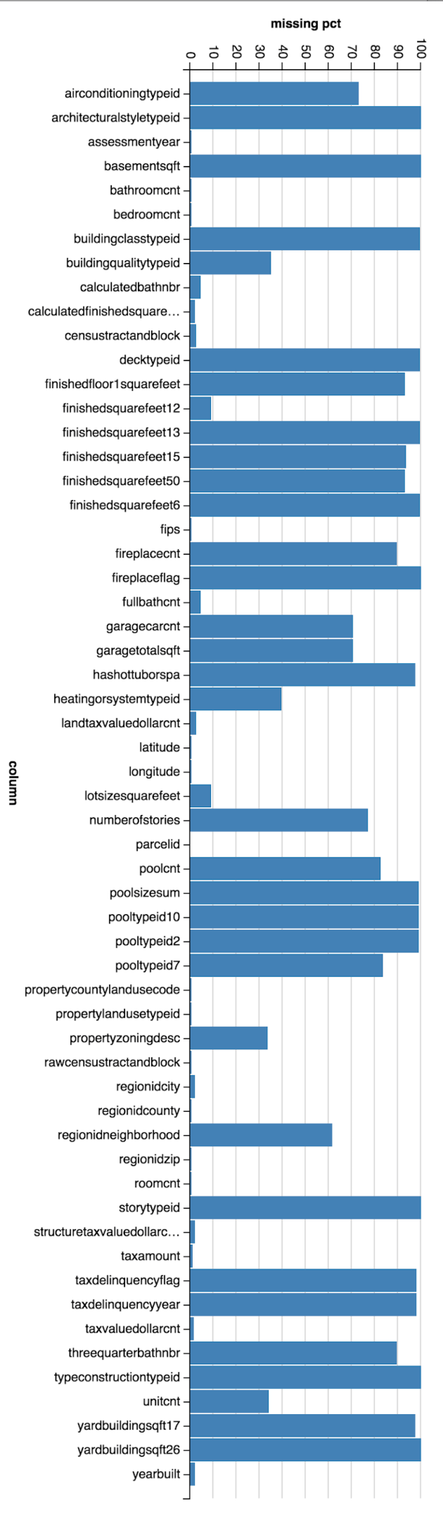
Example usage using Zillow Price Kaggle dataset:


val imputer = new Imputer()
imputer.setInputCols(Array("bedroomcnt", "bathroomcnt", "roomcnt", "calculatedfinishedsquarefeet", "taxamount", "taxvaluedollarcnt", "landtaxvaluedollarcnt", "structuretaxvaluedollarcnt")) 

imputer.setOutputCols(Array("bedroomcnt_out", "bathroomcnt_out", "roomcnt_out", "calculatedfinishedsquarefeet_out", "taxamount_out", "taxvaluedollarcnt_out", "landtaxvaluedollarcnt_out", "structuretaxvaluedollarcnt_out"))
   

However, I ran into this issue, it can’t handle column values of integer type. See this Jira ticket.

https://issues.apache.org/jira/browse/SPARK-20604

The good news is a pull request was created to fix the issue by converting integer type to double type during imputation. See the pull request below.

https://github.com/apache/spark/pull/17864

Zillow Price Kaggle Competition Part 2

From my last blog, I calculated the missing value percentage for every columns in the data. Next thing to do is to perform imputation of missing values in selected columns before model training.

However, I am going to skip doing in depth data cleaning and feature selection eg. removing outliers and calculating correlations between features, etc. I will do that in the next blog 😉

Instead I am going to use  the following features to build a model. These columns have low missing value percentage.

"bedroomcnt"
"bathroomcnt"
"roomcnt"
"taxamount"
"taxvaluedollarcnt"
"lotsizesquarefeet"
"finishedsquarefeet12"
"latitude"
"longitude"

I replaced missing values in bedroomcnt with 3 and bathroomcnt with 2 (use most frequent value) and drop any row that has any missing values in the other columns.

In this experiment, I used Spark to train a Gradient Boost Tree Regression model. I built a Spark ML pipeline to perform hyperparameter tuning of GBT. Basically, it will test a grid of different hyperparameters and choose the best parameters based on the evaluation metric, RMSE.

val paramGrid = new ParamGridBuilder()
      .addGrid(gbt.maxDepth, Array(2,5))
      .addGrid(gbt.maxIter, Array(50,100))
      .build()


Screen Shot 2017-08-07 at 12.37.39 AM

Screen Shot 2017-08-07 at 12.42.14 AM

Next I will need to go back to data cleaning and feature selection to choose better/more features to improve the model.

Zillow Prize Kaggle Competition: Exploratory Analysis Part 1

You can download the Zillow Price Kaggle datasets from https://www.kaggle.com/c/zillow-prize-1
For this exploratory study of property dataset, I used Spark to calculate the missing value percentage for each column. As you can see below, as many as 20 columns have greater than 90% null/empty values. Examples: storytypeid, basementsqft, yardbuildingsqft.

(Column Name, Missing Value Percentage)
(storytypeid,99.94559859467502)
(basementsqft,99.94546460106585)
(yardbuildingsqft26,99.91132972912857)
(fireplaceflag,99.82704774895761)
(architecturalstyletypeid,99.79696618369786)
(typeconstructiontypeid,99.7739862797244)
(finishedsquarefeet13,99.74300025760272)
(buildingclasstypeid,99.57694867743282)
(decktypeid,99.42731131438686)
(finishedsquarefeet6,99.26300165113625)
(poolsizesum,99.06338467186806)
(pooltypeid2,98.92553874642948)
(pooltypeid10,98.76260251767292)
(taxdelinquencyflag,98.10861320969296)
(taxdelinquencyyear,98.10854621288838)
(hashottuborspa,97.68814126410241)
(yardbuildingsqft17,97.30823588368953)
(finishedsquarefeet15,93.60857183916613)
(finishedfloor1squarefeet,93.20930438222749)
(finishedsquarefeet50,93.20930438222749)

(threequarterbathnbr,89.56085939481116)
(fireplacecnt,89.5271600021037)
(pooltypeid7,83.73789912090143)
(poolcnt,82.66343786733091)
(numberofstories,77.15177824593657)
(airconditioningtypeid,72.81541006901676)
(garagecarcnt,70.41196670124819)
(garagetotalsqft,70.41196670124819)
(regionidneighborhood,61.26238059075773)
(heatingorsystemtypeid,39.488452598253325)
(buildingqualitytypeid,35.06374913448503)
(unitcnt,33.75724444822604)
(propertyzoningdesc,33.71908976801352)
(lotsizesquarefeet,9.248875374888994)
(finishedsquarefeet12,9.24666448033761)
(calculatedbathnbr,4.31834603648579)
(fullbathcnt,4.31834603648579)
(censustractandblock,2.5166009707167016)
(landtaxvaluedollarcnt,2.268947282559358)
(regionidcity,2.10520709214774)
(yearbuilt,2.0074922526570096)
(calculatedfinishedsquarefeet,1.8613387234495853)
(structuretaxvaluedollarcnt,1.8418091549123563)
(taxvaluedollarcnt,1.4253570175970458)
(taxamount,1.0468250716782062)
(regionidzip,0.46830766406596236)
(propertycountylandusecode,0.4112598849597868)
(roomcnt,0.3843941663202374)
(bathroomcnt,0.38395868709041925)
(bedroomcnt,0.3835567062628948)
(assessmentyear,0.38318822383766404)
(fips,0.38312122703307666)
(latitude,0.38312122703307666)
(longitude,0.38312122703307666)
(propertylandusetypeid,0.38312122703307666)
(rawcensustractandblock,0.38312122703307666)
(regionidcounty,0.38312122703307666)
(parcelid,0.0)

Screen Shot 2017-08-05 at 12.24.07 AM

Now I have identified the good columns (italics bold, less than 10% empty values) and bad columns. The next step is to determine if we can apply some sorts of missing values imputation to any of those problematic columns.

A few missing value imputation techniques are available, such as using mean, median, or most frequent value as replacement value.

InstaCart: Product Recommender

InstaCart has recently open sourced anonymized data on customer orders for its Kaggle competition. You can find out more info from the link below.

https://www.kaggle.com/c/instacart-market-basket-analysis

Previously, I did some data exploration to discover some interesting insights. See my previous blog post.

Next I would like to use their anonymized data to build a product recommender system. There are many approaches/strategies in product recommendations, eg. Most popular items, Also bought/viewed, Featured items, and etc. I am going to explore the most popular items approach and collaborative filtering (also bought) approach.

We can identify the top 5 popular items for each department and utilize them for most popular items recommendation. For example, the top 5 items for frozen department are Blueberries, Organic Broccoli Florets, Organic Whole Strawberries, Pipeapple Chunks, Frozen Organic Wild Blueberries.

Screen Shot 2017-07-10 at 10.51.55 PM

Next, I utilized Spark ALS algorithm to  build a collaborative filtering based recommender system.

Some stats about the data

Total user-product pair (rating): 1,384,617

Total users: 131,209

Total products: 39,123

Given the data, I splitted the data into train set (0.8) vs test set (0.2) randomly. This resulted in
Number of train elements: 1,107,353
Number of test elements: 277,264

Here are the parameters I used in ALS, rank = 10, lambda = 1, number of iterations = 10, 50, 60, 80

  • Number of iterations = 10,    RMSE = 0.9999895
  • Number of iterations = 50,    RMSE = 0.9999828
  • Number of iterations = 60,    RMSE = 0.9999875
  • Number of iterations = 80,    RMSE = 0.9999933

We can also try out different ranks in grid search.

Here are some recommendations suggested by ALS collaborative filtering algorithm (number of iterations =80, rank=10)

Given user 124383 Transaction History

+——-+———-+—–+———-+—————————+——–+————-+
|user_id|product_id|count|product_id|product_name |aisle_id|department_id|
+——-+———-+—–+———-+—————————+——–+————-+
|124383 |49478 |1 |49478 |Frozen Organic Strawberries|24 |4 |
|124383 |21903 |1 |21903 |Organic Baby Spinach |123 |4 |
|124383 |19508 |1 |19508 |Corn Tortillas |128 |3 |
|124383 |20114 |1 |20114 |Jalapeno Peppers |83 |4 |
|124383 |44142 |1 |44142 |Red Onion |83 |4 |
|124383 |20345 |1 |20345 |Thin Crust Pepperoni Pizza |79 |1 |
|124383 |27966 |1 |27966 |Organic Raspberries |123 |4 |
+——-+———-+—–+———-+—————————+——–+——————+

Here are the recommendations
+———-+————————————————————-+——–+————-+
|product_id|product_name |aisle_id|department_id|
+———-+————————————————————-+——–+——————+
|28717 |Sport Deluxe Adjustable Black Ankle Stabilizer |133 |11 |
|15372 |Meditating Cedarwood Mineral Bath |25 |11 |
|18962 |Arroz Calasparra Paella Rice |63 |9 |
|2528 |Cluckin’ Good Stew |40 |8 |
|21156 |Dreamy Cold Brew Concentrate |90 |7 |
|12841 |King Crab Legs |39 |12 |
|24862 |Old Indian Wild Cherry Bark Syrup |47 |11 |
|37535 |Voluminous Extra-Volume Collagen Mascara – Blackest Black 680|132 |11 |
|30847 |Wild Oregano Oil |47 |11 |
+———-+————————————————————-+——–+————-+


Analyzing Bike Share Data

In this series, I am going to use Spark to analyze the Bay Area’s Bike Share Data. You can download the dataset from http://www.bayareabikeshare.com/open-data

First let’s find out the top popular start terminals

trips.groupBy("Start Terminal", "Start Station").count().sort(desc("count")).show(false)

screen-shot-2016-12-04-at-9-47-09-am

San Francisco Caltrain (Townsend at 4th) and San Francisco Caltrain 2 (330 Townsend) are the two most popular bike stations. It shows that many Caltrain commuters are using these bikes to travel to their workplaces.

Lets figure out the day of week distribution of trips. As seen below, Thursday, Tuesday are the top two busiest days. It looks like people are most likely to show up at work on Thursday and Tuesday 🙂

On the other hand, Monday has the lowest number of trips among all weekdays. So if you want to have a good meeting attendance, you would probably schedule it on Tuesday or Thursday and try to avoid Monday 🙂

sqlContext.sql("select getDayAsString(day_of_week) as day, count(1) as count from (select `Start Terminal`, `Start Station`, getDayOfWeek(`Start Date`) as day_of_week from trips) as A group by day_of_week order by count desc")

screen-shot-2016-12-04-at-10-04-48-am

Next, lets take a look at the time of day distribution of the trips.

5 PM, 8 AM, 4 PM, 9 AM, 6 PM, 12 AM are the top 6 busiest hours. As expected, the bike usage peaks during morning and evening rush hours as people get to/off work. One interesting observation is the number of bike trips is also high during midnight, ranked sixth in the list.

screen-shot-2016-12-04-at-10-36-47-am

Hmm…I wonder which are the popular stations during morning rush hours from 8 am to 9 am.  As it turns out, San Francisco Caltrain, Temporary Transbay Terminal,  and San Francisco Caltrain 2 are the busiest bike stations during morning rush hours.

screen-shot-2016-12-04-at-11-07-46-am

Since midnight has the fifth highest number of bike trips, lets find out where the top originating bike stations are.

Harry Bridges Plaza (Ferry Building), Embarcadero at Sansome, Market at Sansome, Market at 4th, 2nd at Townsend are among the popular bike stations during midnight hour. See the below list. They are in close proximity to the city popular nightlife hangouts/hotspots.

screen-shot-2016-12-04-at-3-27-11-pm

Lets plot the hourly average bike availability for the top three start stations, San Francisco Caltrain (Townsend at 4th) terminal id 70, San Francisco Caltrain 2 (330 Townsend) terminal id 69, and Harry Bridges Plaza (Ferry Building) terminal id 50

They all share the same pattern, decreasing number of available bikes around morning rush hour, 8 am to 10 am.

screen-shot-2016-12-06-at-9-08-53-pm

Next, lets build a model to predict the bike availability.

To be continued…


Spark: Analyzing Stock Price

Simple moving average is an indicator many people use in analyzing stock price. Here I want to show how to use Spark’s window function to compute the moving average easily.

First, lets load the stock data

import org.apache.spark.sql.expressions.Window
import org.apache.spark.sql.functions._

case class Stock(exc: String, symbol: String, stockDate: String, open: Double, high: Double, low: Double, close: Double,
                   volume: Double, adjClose: Double)

  val data = sc.textFile("s3://giantify-stocks/APC_2016_08_03.csv")
  val stocksData = data.map { d =>
    val tokens = d.split(",")
    Stock(tokens(0), tokens(1), tokens(2), tokens(3).toDouble, tokens(4).toDouble, tokens(5).toDouble, tokens(6).toDouble, tokens(7).toDouble,
      tokens(8).toDouble)
  }.toDF.cache()

  val stocks = stocksData.withColumn("stockDate", to_date(col("stockDate")))

Next we will compute the 20 days, 50 days, 100 days simple moving averages

val movingAverageWindow20 = Window.orderBy("stockDate").rowsBetween(-20, 0)
val movingAverageWindow50 = Window.orderBy("stockDate").rowsBetween(-50, 0)
val movingAverageWindow100 = Window.orderBy("stockDate").rowsBetween(-100, 0)

// Calculate the moving average
val stocksMA = stocks.withColumn( "MA20", avg(stocks("close")).over(movingAverageWindow20)).withColumn( "MA50", avg(stocks("close")).over(movingAverageWindow50)).withColumn("MA100", avg(stocks("close")).over(movingAverageWindow100))

stocksMA.show()

stocksMA.filter("close > MA50").select(col("stockDate"), col("close"), col("MA50")).show()

With the moving average calculated, let’s find when closing price exceeds the 50 days moving average

stocksMA.filter("close > MA50").select(col("stockDate"), col("close"), col("MA50")).show()
Screen Shot 2016-08-21 at 11.29.13 AM

Stay tuned for the next blog on how to use Zeppelin to visualize the price data