Zillow Price Kaggle Competition Part 2

From my last blog, I calculated the missing value percentage for every columns in the data. Next thing to do is to perform imputation of missing values in selected columns before model training.

However, I am going to skip doing in depth data cleaning and feature selection eg. removing outliers and calculating correlations between features, etc. I will do that in the next blog 😉

Instead I am going to use  the following features to build a model. These columns have low missing value percentage.

"bedroomcnt"
"bathroomcnt"
"roomcnt"
"taxamount"
"taxvaluedollarcnt"
"lotsizesquarefeet"
"finishedsquarefeet12"
"latitude"
"longitude"

I replaced missing values in bedroomcnt with 3 and bathroomcnt with 2 (use most frequent value) and drop any row that has any missing values in the other columns.

In this experiment, I used Spark to train a Gradient Boost Tree Regression model. I built a Spark ML pipeline to perform hyperparameter tuning of GBT. Basically, it will test a grid of different hyperparameters and choose the best parameters based on the evaluation metric, RMSE.

val paramGrid = new ParamGridBuilder()
      .addGrid(gbt.maxDepth, Array(2,5))
      .addGrid(gbt.maxIter, Array(50,100))
      .build()


Screen Shot 2017-08-07 at 12.37.39 AM

Screen Shot 2017-08-07 at 12.42.14 AM

Next I will need to go back to data cleaning and feature selection to choose better/more features to improve the model.

Instacart Data Insight

InstaCart has recently organized a Kaggle competition and published anonymized data on customer orders over time to predict which previously purchased products will be in a user’s next order. You can check out the link below.

https://www.kaggle.com/c/instacart-market-basket-analysis

First, I used Spark to analyze the data to uncover hidden insights.

We were given the departments data

Screen Shot 2017-07-05 at 10.04.34 PM

Products data

Screen Shot 2017-07-05 at 10.07.32 PM

Orders data

Screen Shot 2017-07-05 at 10.07.47 PM

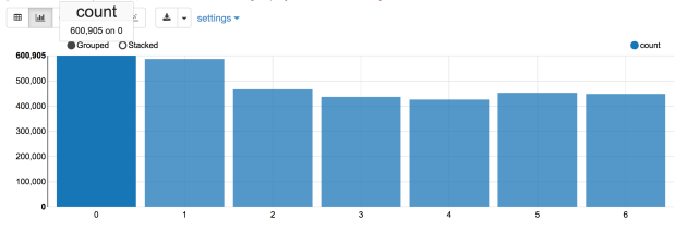
Lets find out which is the busiest day of the week. As it turns out, day 0 is the busiest day, with 600,905 orders followed by day 1 with 587478 orders. I would assume day 0 is Sunday and day 1 is Monday.

Screen Shot 2017-07-05 at 10.15.12 PM.png

Next, lets figure out which is the busiest hour in a day. It turns out 10 am is the busiest hour with 288,418 orders, followed by 11 am with 284,728 orders.

As you can see, Instacart customers like to shop from 11 am to 5 pm. It would be interesting to see the day of week + hour of day breakdown too.

Screen Shot 2017-07-05 at 10.18.24 PM

Here is the breakdown of popular hours for each day. 10 am dominates the top spot.

Screen Shot 2017-07-06 at 12.59.15 AM

Next lets figure out the top ten popular items among Instacart customers. Surprisingly, banana is the most popular item.

Screen Shot 2017-07-05 at 10.09.13 PM.png

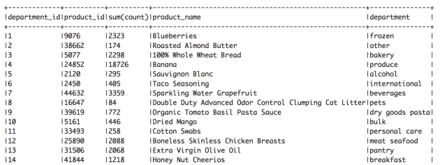
Lets find out the top item for each department. We can see that Blueberries is the most popular item for frozen department and Extra Virgin Olive Oil is the most popular item for pantry department. Some unexpected surprises are dried mango, cotton swabs, and honey nut cheerios.

Screen Shot 2017-07-10 at 10.18.57 PM

We are also interested in knowing the reorder interval, how many days since the prior order before making the next order.

Screen Shot 2017-07-05 at 11.47.04 PM.png

As we discovered, 30 days is the most frequent reorder interval. It looks like most of customers reorder once a month. On the other hand, 320,608 orders were placed after 7 days since the prior order. We can concluded that majority of customers reorder after 1 month or 1 week since the prior order.

Stay tuned for next blog on my study results at the individual user level.

HyperLogLog Aproximate Distinct Counting

In MapReduce, distinct/unique count of large data set is very common but unfortunately it is not scalable because it requires one reducer. It gets worse when you have to perform unique count across different aggregation/segment groups. Again, unique counting across different aggregation granularities whether in terms of time dimension or in combination with other demographic attributes is a common practice in big data analytics. Eg. In your massive data sets, let’s find unique counts of users for every hour, every day, every week, every month and etc.

HyperLogLog approximate unique counting can be used to provide a scalable solution. Keep in mind, the unique count here is a probabilistic approximate counts.You can implement either a map side hyperloglog counting or reduce side hyperloglog counting. However, map side counting requires more memory and beware of out of memory issue if you have many segments to perform unique count on.

For more information, you can check out the following pages

http://highscalability.com/blog/2012/4/5/big-data-counting-how-to-count-a-billion-distinct-objects-us.html

http://stefanheule.com/papers/edbt2013-hyperloglog.pdf

http://tech.adroll.com/media/hllminhash.pdf

http://www.looker.com/news/blog/practical-data-science-amazon-announces-hyperloglog