Instacart Data Insight

InstaCart has recently organized a Kaggle competition and published anonymized data on customer orders over time to predict which previously purchased products will be in a user’s next order. You can check out the link below.

https://www.kaggle.com/c/instacart-market-basket-analysis

First, I used Spark to analyze the data to uncover hidden insights.

We were given the departments data

Screen Shot 2017-07-05 at 10.04.34 PM

Products data

Screen Shot 2017-07-05 at 10.07.32 PM

Orders data

Screen Shot 2017-07-05 at 10.07.47 PM

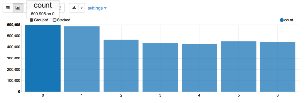
Lets find out which is the busiest day of the week. As it turns out, day 0 is the busiest day, with 600,905 orders followed by day 1 with 587478 orders. I would assume day 0 is Sunday and day 1 is Monday.

Screen Shot 2017-07-05 at 10.15.12 PM.png

Next, lets figure out which is the busiest hour in a day. It turns out 10 am is the busiest hour with 288,418 orders, followed by 11 am with 284,728 orders.

As you can see, Instacart customers like to shop from 11 am to 5 pm. It would be interesting to see the day of week + hour of day breakdown too.

Screen Shot 2017-07-05 at 10.18.24 PM

Here is the breakdown of popular hours for each day. 10 am dominates the top spot.

Screen Shot 2017-07-06 at 12.59.15 AM

Next lets figure out the top ten popular items among Instacart customers. Surprisingly, banana is the most popular item.

Screen Shot 2017-07-05 at 10.09.13 PM.png

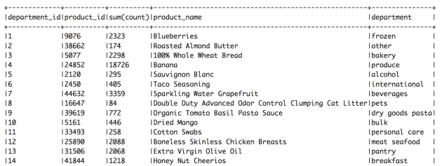
Lets find out the top item for each department. We can see that Blueberries is the most popular item for frozen department and Extra Virgin Olive Oil is the most popular item for pantry department. Some unexpected surprises are dried mango, cotton swabs, and honey nut cheerios.

Screen Shot 2017-07-10 at 10.18.57 PM

We are also interested in knowing the reorder interval, how many days since the prior order before making the next order.

Screen Shot 2017-07-05 at 11.47.04 PM.png

As we discovered, 30 days is the most frequent reorder interval. It looks like most of customers reorder once a month. On the other hand, 320,608 orders were placed after 7 days since the prior order. We can concluded that majority of customers reorder after 1 month or 1 week since the prior order.

Stay tuned for next blog on my study results at the individual user level.

Spark: Analyzing Stock Price

Simple moving average is an indicator many people use in analyzing stock price. Here I want to show how to use Spark’s window function to compute the moving average easily.

First, lets load the stock data

import org.apache.spark.sql.expressions.Window
import org.apache.spark.sql.functions._

case class Stock(exc: String, symbol: String, stockDate: String, open: Double, high: Double, low: Double, close: Double,
                   volume: Double, adjClose: Double)

  val data = sc.textFile("s3://giantify-stocks/APC_2016_08_03.csv")
  val stocksData = data.map { d =>
    val tokens = d.split(",")
    Stock(tokens(0), tokens(1), tokens(2), tokens(3).toDouble, tokens(4).toDouble, tokens(5).toDouble, tokens(6).toDouble, tokens(7).toDouble,
      tokens(8).toDouble)
  }.toDF.cache()

  val stocks = stocksData.withColumn("stockDate", to_date(col("stockDate")))

Next we will compute the 20 days, 50 days, 100 days simple moving averages

val movingAverageWindow20 = Window.orderBy("stockDate").rowsBetween(-20, 0)
val movingAverageWindow50 = Window.orderBy("stockDate").rowsBetween(-50, 0)
val movingAverageWindow100 = Window.orderBy("stockDate").rowsBetween(-100, 0)

// Calculate the moving average
val stocksMA = stocks.withColumn( "MA20", avg(stocks("close")).over(movingAverageWindow20)).withColumn( "MA50", avg(stocks("close")).over(movingAverageWindow50)).withColumn("MA100", avg(stocks("close")).over(movingAverageWindow100))

stocksMA.show()

stocksMA.filter("close > MA50").select(col("stockDate"), col("close"), col("MA50")).show()

With the moving average calculated, let’s find when closing price exceeds the 50 days moving average

stocksMA.filter("close > MA50").select(col("stockDate"), col("close"), col("MA50")).show()
Screen Shot 2016-08-21 at 11.29.13 AM

Stay tuned for the next blog on how to use Zeppelin to visualize the price data

Stock Clustering

Diversification in stock portfolio is always desired to minimize the risk. One of the many ways is to cluster these stocks into many categories in which each category exhibits similar behavior.

Here are a few categories I identified with some stocks by applying simple clustering algorithm.

Category 1


Screen Shot 2015-12-25 at 9.32.29 PM

Screen Shot 2015-12-25 at 9.33.47 PM

Category 2:

Screen Shot 2015-12-25 at 9.47.56 PM

Screen Shot 2015-12-25 at 9.49.17 PM

Category 3:

Screen Shot 2015-12-25 at 9.50.31 PM.png

Screen Shot 2015-12-25 at 9.53.13 PM

Category 4:

Screen Shot 2015-12-25 at 9.55.56 PM

Screen Shot 2015-12-25 at 9.56.46 PM

In the experiment, I tried with different number of clusters and calculated its corresponding cost. See the following chart, I chose 15 as the ideal number of clusters to cluster 93 stocks I have in the portfolio.

Screen Shot 2015-12-25 at 10.09.34 PM

The main goal of this exercise is to build a balanced portfolio with combination of stocks from different categories to minimize risk.

Disclaimer: Trading is risky and you can lose all money. Past performance is not a guide to future performance. The content is intended to be used and must be used for informational purposes only. It is very important to do your own analysis and consult a financial professional’s advice to verify our content. It is very important to do your own analysis before making any investment based on your own personal circumstances.

Randomness in Random Forest

In the last post, we looked at the bagging process where a random sample of input is used to build each individual tree. This is one of the two types of randomness used in the algorithm. The second kind of randomness is used in the node splitting process. During the process, a random set of m attributes out of all attributes is used to compute the best split based on information gain.

If m is not specified in the algorithm, then the following logic is used to determine m.

For regression tree,

m = (int) Math.ceil(total_number_attributes / 3.0);

For classification tree,

m = (int) Math.ceil(Math.sqrt(total_number_attributes));

If you take a look at the Apache Mahout DecisionTreeBuilder, you will find the randomAttributes method below. This method selects m attributes to consider for split.

org.apache.mahout.classifier.df.builder.DecisionTreeBuilder

/**
   * Randomly selects m attributes to consider for split, excludes IGNORED and LABEL attributes
   *
   * @param rng      random-numbers generator
   * @param selected attributes' state (selected or not)
   * @param m        number of attributes to choose
   * @return list of selected attributes' indices, or null if all attributes have already been selected
   */
  private static int[] randomAttributes(Random rng, boolean[] selected, int m) {
    int nbNonSelected = 0; // number of non selected attributes
    for (boolean sel : selected) {
      if (!sel) {
        nbNonSelected++;
      }
    }

    if (nbNonSelected == 0) {
      log.warn("All attributes are selected !");
      return NO_ATTRIBUTES;
    }

    int[] result;
    if (nbNonSelected <= m) {
      // return all non selected attributes
      result = new int[nbNonSelected];
      int index = 0;
      for (int attr = 0; attr < selected.length; attr++) {
        if (!selected[attr]) {
          result[index++] = attr;
        }
      }
    } else {
      result = new int[m];
      for (int index = 0; index < m; index++) {
        // randomly choose a "non selected" attribute
        int rind;
        do {
          rind = rng.nextInt(selected.length);
        } while (selected[rind]);

        result[index] = rind;
        selected[rind] = true; // temporarily set the chosen attribute to be selected
      }

      // the chosen attributes are not yet selected
      for (int attr : result) {
        selected[attr] = false;
      }
    }

    return result;
  }

Given the list of chosen attributes, it loops through each one and computes the information gains for different splits generated by using different attributes and try to find the best split.


 // find the best split
    Split best = null;
    for (int attr : attributes) {
      Split split = igSplit.computeSplit(data, attr);
      if (best == null || best.getIg() < split.getIg()) {
        best = split;
      }
    }

After getting the best split, if the information gain is less than the specified threshold, then we stop and create the leaf node with the label.
For regression, the label is the regression value which is calculated by taking the average of all the values of the sample data set. For classification, we use the majority label, the value that appears the most.

 // information gain is near to zero.
    if (best.getIg() < EPSILON) {
      double label;
      if (data.getDataset().isNumerical(data.getDataset().getLabelId())) {
        label = sum / data.size();
      } else {
        label = data.majorityLabel(rng);
      }
      log.debug("ig is near to zero Leaf({})", label);
      return new Leaf(label);
    }

HyperLogLog vs LogLog

To understand HyperLogLog (HLL), one should read the LogLog and HyperLogLog papers.

http://algo.inria.fr/flajolet/Publications/DuFl03-LNCS.pdf  (LogLog)

http://algo.inria.fr/flajolet/Publications/FlFuGaMe07.pdf  (HyperLogLog)

The major difference between the two is one uses regular mean and the other (HLL) uses harmonic mean to average the estimate cardinality calculated by different m buckets. I would view these buckets as different experiments.

The accuracy (standard error) is controlled by the number of buckets, m. The more buckets the better is the estimation. But, HLL has better accuracy compared to LogLog given the same number of buckets.

The standard error for HLL is

CodeCogsEqn


The standard error for LogLog is

CodeCogsEqn (1)

The following is the LogLog algorithm taken from the paper

Screen shot 2014-07-29 at 8.07.49 PM

Basically, there are m buckets, each one is keeping track of the run of consecutive zeros in the bit string. We then figure out the max run of consecutive zeros (position of leftmost 1) in all the buckets.

eg.  1  => 1,   001 =>3

Then using the cardinality estimate formula shown in the last line, calculate the estimate unique counts. As you see from the formula, it involves taking the average of the run of zeros observed in these buckets. (Note: the alpha is the bias correction applied to the cardinality estimate)

For HyperLogLog, instead of using the average, harmonic mean (stochastic averaging) is used. Please refer to the HLL paper for more detailed description of the formula.

Taken from the HLL paper,

Screen shot 2014-07-29 at 8.24.19 PM

HyperLogLog Aproximate Distinct Counting

In MapReduce, distinct/unique count of large data set is very common but unfortunately it is not scalable because it requires one reducer. It gets worse when you have to perform unique count across different aggregation/segment groups. Again, unique counting across different aggregation granularities whether in terms of time dimension or in combination with other demographic attributes is a common practice in big data analytics. Eg. In your massive data sets, let’s find unique counts of users for every hour, every day, every week, every month and etc.

HyperLogLog approximate unique counting can be used to provide a scalable solution. Keep in mind, the unique count here is a probabilistic approximate counts.You can implement either a map side hyperloglog counting or reduce side hyperloglog counting. However, map side counting requires more memory and beware of out of memory issue if you have many segments to perform unique count on.

For more information, you can check out the following pages

http://highscalability.com/blog/2012/4/5/big-data-counting-how-to-count-a-billion-distinct-objects-us.html

http://stefanheule.com/papers/edbt2013-hyperloglog.pdf

http://tech.adroll.com/media/hllminhash.pdf

http://www.looker.com/news/blog/practical-data-science-amazon-announces-hyperloglog