g2.8xlarge does not support NVIDIA GPUDirect peer to peer transfers

Go to

/home/ubuntu/NVIDIA_CUDA-8.0_Samples/0_Simple/simpleP2P

run make and then execute

./simpleP2P

[./simpleP2P] – Starting…
Checking for multiple GPUs…
CUDA-capable device count: 4
> GPU0 = ” GRID K520″ IS capable of Peer-to-Peer (P2P)
> GPU1 = ” GRID K520″ IS capable of Peer-to-Peer (P2P)
> GPU2 = ” GRID K520″ IS capable of Peer-to-Peer (P2P)
> GPU3 = ” GRID K520″ IS capable of Peer-to-Peer (P2P)

Checking GPU(s) for support of peer to peer memory access…
> Peer access from GRID K520 (GPU0) -> GRID K520 (GPU1) : No
> Peer access from GRID K520 (GPU0) -> GRID K520 (GPU2) : No
> Peer access from GRID K520 (GPU0) -> GRID K520 (GPU3) : No
> Peer access from GRID K520 (GPU1) -> GRID K520 (GPU0) : No
> Peer access from GRID K520 (GPU1) -> GRID K520 (GPU2) : No
> Peer access from GRID K520 (GPU1) -> GRID K520 (GPU3) : No
> Peer access from GRID K520 (GPU2) -> GRID K520 (GPU0) : No
> Peer access from GRID K520 (GPU2) -> GRID K520 (GPU1) : No
> Peer access from GRID K520 (GPU2) -> GRID K520 (GPU3) : No
> Peer access from GRID K520 (GPU3) -> GRID K520 (GPU0) : No
> Peer access from GRID K520 (GPU3) -> GRID K520 (GPU1) : No
> Peer access from GRID K520 (GPU3) -> GRID K520 (GPU2) : No
Two or more GPUs with SM 2.0 or higher capability are required for ./simpleP2P.
Peer to Peer access is not available amongst GPUs in the system, waiving test.

As you can see, g2.8xlarge does not support NVIDIA GPUDirect peer to peer transfers. Only P2 instances have the support.

Analyzing Bike Share Data

In this series, I am going to use Spark to analyze the Bay Area’s Bike Share Data. You can download the dataset from http://www.bayareabikeshare.com/open-data

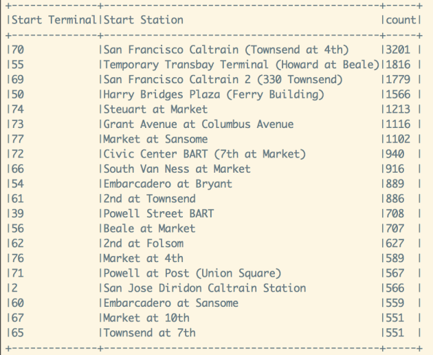
First let’s find out the top popular start terminals

trips.groupBy("Start Terminal", "Start Station").count().sort(desc("count")).show(false)

screen-shot-2016-12-04-at-9-47-09-am

San Francisco Caltrain (Townsend at 4th) and San Francisco Caltrain 2 (330 Townsend) are the two most popular bike stations. It shows that many Caltrain commuters are using these bikes to travel to their workplaces.

Lets figure out the day of week distribution of trips. As seen below, Thursday, Tuesday are the top two busiest days. It looks like people are most likely to show up at work on Thursday and Tuesday 🙂

On the other hand, Monday has the lowest number of trips among all weekdays. So if you want to have a good meeting attendance, you would probably schedule it on Tuesday or Thursday and try to avoid Monday 🙂

sqlContext.sql("select getDayAsString(day_of_week) as day, count(1) as count from (select `Start Terminal`, `Start Station`, getDayOfWeek(`Start Date`) as day_of_week from trips) as A group by day_of_week order by count desc")

screen-shot-2016-12-04-at-10-04-48-am

Next, lets take a look at the time of day distribution of the trips.

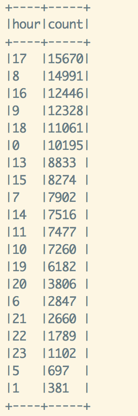
5 PM, 8 AM, 4 PM, 9 AM, 6 PM, 12 AM are the top 6 busiest hours. As expected, the bike usage peaks during morning and evening rush hours as people get to/off work. One interesting observation is the number of bike trips is also high during midnight, ranked sixth in the list.

screen-shot-2016-12-04-at-10-36-47-am

Hmm…I wonder which are the popular stations during morning rush hours from 8 am to 9 am.  As it turns out, San Francisco Caltrain, Temporary Transbay Terminal,  and San Francisco Caltrain 2 are the busiest bike stations during morning rush hours.

screen-shot-2016-12-04-at-11-07-46-am

Since midnight has the fifth highest number of bike trips, lets find out where the top originating bike stations are.

Harry Bridges Plaza (Ferry Building), Embarcadero at Sansome, Market at Sansome, Market at 4th, 2nd at Townsend are among the popular bike stations during midnight hour. See the below list. They are in close proximity to the city popular nightlife hangouts/hotspots.

screen-shot-2016-12-04-at-3-27-11-pm

Lets plot the hourly average bike availability for the top three start stations, San Francisco Caltrain (Townsend at 4th) terminal id 70, San Francisco Caltrain 2 (330 Townsend) terminal id 69, and Harry Bridges Plaza (Ferry Building) terminal id 50

They all share the same pattern, decreasing number of available bikes around morning rush hour, 8 am to 10 am.

screen-shot-2016-12-06-at-9-08-53-pm

Next, lets build a model to predict the bike availability.

To be continued…


Spark: Analyzing Stock Price

Simple moving average is an indicator many people use in analyzing stock price. Here I want to show how to use Spark’s window function to compute the moving average easily.

First, lets load the stock data

import org.apache.spark.sql.expressions.Window
import org.apache.spark.sql.functions._

case class Stock(exc: String, symbol: String, stockDate: String, open: Double, high: Double, low: Double, close: Double,
                   volume: Double, adjClose: Double)

  val data = sc.textFile("s3://giantify-stocks/APC_2016_08_03.csv")
  val stocksData = data.map { d =>
    val tokens = d.split(",")
    Stock(tokens(0), tokens(1), tokens(2), tokens(3).toDouble, tokens(4).toDouble, tokens(5).toDouble, tokens(6).toDouble, tokens(7).toDouble,
      tokens(8).toDouble)
  }.toDF.cache()

  val stocks = stocksData.withColumn("stockDate", to_date(col("stockDate")))

Next we will compute the 20 days, 50 days, 100 days simple moving averages

val movingAverageWindow20 = Window.orderBy("stockDate").rowsBetween(-20, 0)
val movingAverageWindow50 = Window.orderBy("stockDate").rowsBetween(-50, 0)
val movingAverageWindow100 = Window.orderBy("stockDate").rowsBetween(-100, 0)

// Calculate the moving average
val stocksMA = stocks.withColumn( "MA20", avg(stocks("close")).over(movingAverageWindow20)).withColumn( "MA50", avg(stocks("close")).over(movingAverageWindow50)).withColumn("MA100", avg(stocks("close")).over(movingAverageWindow100))

stocksMA.show()

stocksMA.filter("close > MA50").select(col("stockDate"), col("close"), col("MA50")).show()

With the moving average calculated, let’s find when closing price exceeds the 50 days moving average

stocksMA.filter("close > MA50").select(col("stockDate"), col("close"), col("MA50")).show()
Screen Shot 2016-08-21 at 11.29.13 AM

Stay tuned for the next blog on how to use Zeppelin to visualize the price data

Useful Spark Code Snippets for Data Analytics

Here are some Spark code snippets you will find particularly useful when performing basic big data analytics

Read CSV

import com.databricks.spark.csv._
val data = sqlContext.read.format("com.databricks.spark.csv").option("header","true").option("inferSchema","true").load(YOUR_INPUT_PATH)

Read AVRO

import com.databricks.spark.avro._
val data = sqlContext.read.avro(YOUR_INPUT_PATH)

Read JSON

val data = sqlContext.read.json(YOUR_INPUT_PATH)

Most often or not, you will probably perform some aggregations

val result = data.groupBy("company_branch").count().sort(desc("count"))
val result = data.groupBy("company_branch", "department").count().sort(asc("company_branch"),desc("count"))

You would want to save your results back to CSV file again

result.write.format("com.databricks.spark.csv").save(YOUR_OUTPUT_PATH)

If you want to consolidate all the result part files into one single file, you can use the coalesce(1) method

result.coalesce(1).write.format("com.databricks.spark.csv").save(YOUR_OUTPUT_PATH)

To perform projection/selection,

data.select(col("name"), col("age"), col("department_name").alias("dept"))

To perform filtering

data.filter("age > 18")

To use SQL, call the registerTempTable method on the dataframe

data.registerTempTable("data")
sqlContext.sql("select name, age from data")

Analyzing Uber Data

Thanks to FiveThirtyEight, we can now play with some New York’s Uber trip datasets (apr 2014 to sept 2014)

https://github.com/fivethirtyeight/uber-tlc-foil-response

I wrote a simple Spark job to analyze the data and create some visualizations using Zeppelin to tell the story from the numbers.

First, lets find out the day of week distribution of New York’s Uber trips. From the table below, we can see that Saturday has the most number of trips, totaled 537,091 followed by Sunday, with 534,856 trips whereas Wednesday has the least number of trips.

Note: dayOfWeek [Saturday: 7, Sunday: 1, Monday: 2, Tuesday:3, Wednesday:4, Thursday:5, Friday:6]


Screen Shot 2016-07-12 at 11.02.50 PM

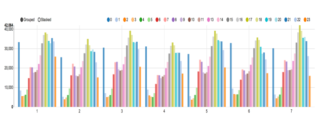
Next, lets study the temporal pattern of Uber trips. With the data, I computed the hour distribution of Uber trips as shown by the bar chart below.

hourDistributionChart

Without no surprise, the number of Uber trips peaked around 5 pm during the evening rush hour period. As we see from the chart, the traffic began to increase from 2pm till 9 pm. A smaller peak was found around morning rush hour from 6 am to 8 am. Another interesting observation is that midnight 12 am also has a significant high number of Uber trips.

Most number of trips at peak hour 5 pm

hour17

Least number of trips at 2 am

hour2


HourDistribution-2

I also created the number of trips vs hour + day of week bar charts shown above to get a better understanding of hour distribution of trips for each of the day of week. Once again I used the following integers mapping to represent different day of week. Each color bar represents the number of Uber trips for the corresponding hour for the specific day of week.

Note: dayOfWeek [Saturday: 7, Sunday: 1, Monday: 2, Tuesday:3, Wednesday:4, Thursday:5, Friday:6]

As we can see from above, for group 2 which represents Monday, we have the least number of midnight trips, (dark blue bar, 0). Most people were going home earlier on Sunday night, resulted in the least number of mid night trips.

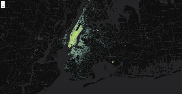
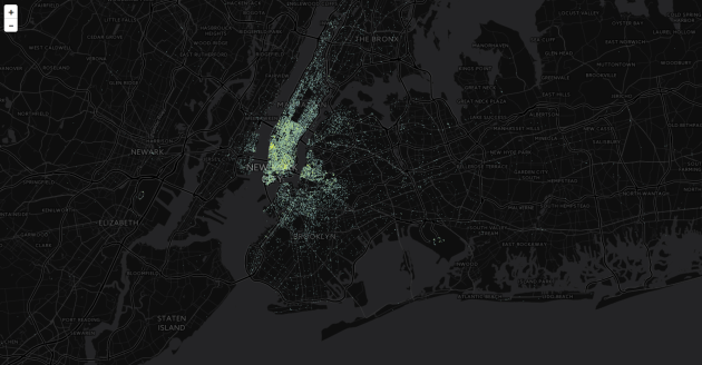
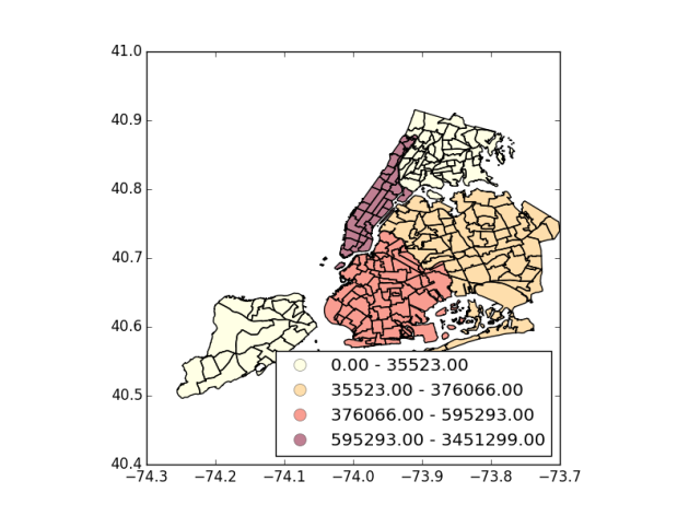
Next question we would like to answer is where are the hot spots with many Uber pickups. Using the NYC Open Data neighborhood shapefile for New York, we can group these pickups location by neighborhood and figure out these hotspots.

Identified popular hotspots

Manhanttan,3451299
Brooklyn, 595293
Queens,376066
Bronx,35522
Staten Island,1982

groupedByBoroOnly

These are the hot neighborhoods with the most Uber’s pickups

1)Manhattan, Midtown-Midtown South
2)Manhattan, Hudson Yards-Chelsea-Flatiron-Union Square
3)Manhattan, SoHo-TriBeCa-Civic Center-Little Italy
4)Manhattan, West Village
5)Manhattan, Turtle Bay-East Midtown
6)Queens, Airport
7)Manhattan, Upper East Side-Carnegie Hill
8)Manhattan, Battery Park City-Lower Manhattan

With the above insights, Uber drivers in New York can know the best days, hours, and locations to get customers.

If we analyze the trend of number of Uber’s pickups over time, from April 2014 to Sept 2014, it is obvious that Uber is getting more and more popular over time.

+——————–+—-+—–+——+
| boro|year|month| count|
+——————–+—-+—–+——+
|Bronx …|2014| 4| 3314|
|Bronx …|2014| 5| 3922|
|Bronx …|2014| 6| 4411|
|Bronx …|2014| 7| 6195|
|Bronx …|2014| 8| 8010|
|Bronx …|2014| 9| 9670|
|Brooklyn …|2014| 4| 61840|
|Brooklyn …|2014| 5| 73608|
|Brooklyn …|2014| 6| 77839|
|Brooklyn …|2014| 7|105489|
|Brooklyn …|2014| 8|129725|
|Brooklyn …|2014| 9|146792|
|Manhattan …|2014| 4|454311|
|Manhattan …|2014| 5|517599|
|Manhattan …|2014| 6|517848|
|Manhattan …|2014| 7|603413|
|Manhattan …|2014| 8|596033|
|Manhattan …|2014| 9|762095|
|Queens …|2014| 4| 37134|
|Queens …|2014| 5| 48948|
|Queens …|2014| 6| 53136|
|Queens …|2014| 7| 67360|
|Queens …|2014| 8| 78675|
|Queens …|2014| 9| 90813|
|Staten Island …|2014| 4| 234|
|Staten Island …|2014| 5| 288|
|Staten Island …|2014| 6| 246|
|Staten Island …|2014| 7| 340|
|Staten Island …|2014| 8| 413|
|Staten Island …|2014| 9| 461|
+——————–+—-+—–+——+


Stock Clustering

Diversification in stock portfolio is always desired to minimize the risk. One of the many ways is to cluster these stocks into many categories in which each category exhibits similar behavior.

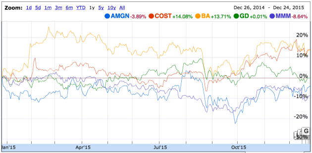
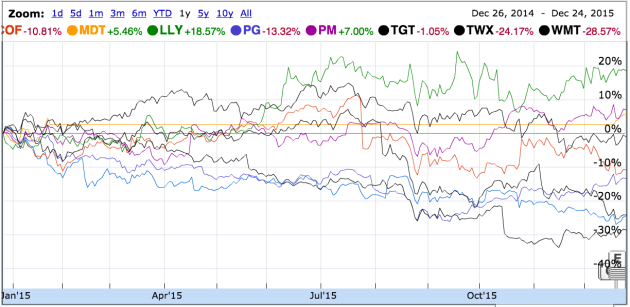
Here are a few categories I identified with some stocks by applying simple clustering algorithm.

Category 1


Screen Shot 2015-12-25 at 9.32.29 PM

Screen Shot 2015-12-25 at 9.33.47 PM

Category 2:

Screen Shot 2015-12-25 at 9.47.56 PM

Screen Shot 2015-12-25 at 9.49.17 PM

Category 3:

Screen Shot 2015-12-25 at 9.50.31 PM.png

Screen Shot 2015-12-25 at 9.53.13 PM

Category 4:

Screen Shot 2015-12-25 at 9.55.56 PM

Screen Shot 2015-12-25 at 9.56.46 PM

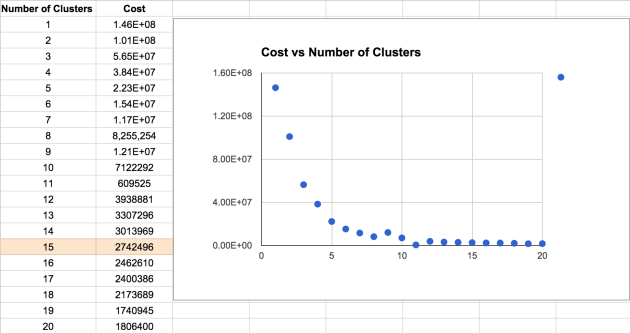
In the experiment, I tried with different number of clusters and calculated its corresponding cost. See the following chart, I chose 15 as the ideal number of clusters to cluster 93 stocks I have in the portfolio.

Screen Shot 2015-12-25 at 10.09.34 PM

The main goal of this exercise is to build a balanced portfolio with combination of stocks from different categories to minimize risk.

Disclaimer: Trading is risky and you can lose all money. Past performance is not a guide to future performance. The content is intended to be used and must be used for informational purposes only. It is very important to do your own analysis and consult a financial professional’s advice to verify our content. It is very important to do your own analysis before making any investment based on your own personal circumstances.

Spark Logistic Regression

Lets dive into the implementation of Logistic Regression in Spark. You can find the implementation in LogisticRegression.scala class. I am looking at the low level mllib library instead of the newer ml API.

/mllib/src/main/scala/org/apache/spark/mllib/classification/LogisticRegression.scala

It defines the LogisticsRegressionModel which extends abstract class GeneralizedLinearModel (/mllib/src/main/scala/org/apache/spark/mllib/regression/GeneralizedLinearAlgorithm.scala) and ClassificationModel, Serializable, Saveable and PMMLExportable traits.

class LogisticRegressionModel @Since("1.3.0") (
    @Since("1.0.0") override val weights: Vector,
    @Since("1.0.0") override val intercept: Double,
    @Since("1.3.0") val numFeatures: Int,
    @Since("1.3.0") val numClasses: Int)
  extends GeneralizedLinearModel(weights, intercept) with ClassificationModel with Serializable
  with Saveable with PMMLExportable {

ClassificationModel defines various predict methods without concrete implementation

trait ClassificationModel extends Serializable {
  /**
   * Predict values for the given data set using the model trained.
   *
   * @param testData RDD representing data points to be predicted
   * @return an RDD[Double] where each entry contains the corresponding prediction
   */
  @Since("1.0.0")
  def predict(testData: RDD[Vector]): RDD[Double]

  /**
   * Predict values for a single data point using the model trained.
   *
   * @param testData array representing a single data point
   * @return predicted category from the trained model
   */
  @Since("1.0.0")
  def predict(testData: Vector): Double

  /**
   * Predict values for examples stored in a JavaRDD.
   * @param testData JavaRDD representing data points to be predicted
   * @return a JavaRDD[java.lang.Double] where each entry contains the corresponding prediction
   */
  @Since("1.0.0")
  def predict(testData: JavaRDD[Vector]): JavaRDD[java.lang.Double] =
    predict(testData.rdd).toJavaRDD().asInstanceOf[JavaRDD[java.lang.Double]]
}

In LogisticRegressionModel’s predictPoint method, if the number of classes is 2 then we have binary classification, otherwise it will perform multinomial logistic regression classification.

 override protected def predictPoint(
      dataMatrix: Vector,
      weightMatrix: Vector,
      intercept: Double) = {
    require(dataMatrix.size == numFeatures)

    // If dataMatrix and weightMatrix have the same dimension, it's binary logistic regression.
    if (numClasses == 2) {
      val margin = dot(weightMatrix, dataMatrix) + intercept
      val score = 1.0 / (1.0 + math.exp(-margin))
      threshold match {
        case Some(t) => if (score > t) 1.0 else 0.0
        case None => score
      }
    } else {
      /**
       * Compute and find the one with maximum margins. If the maxMargin is negative, then the
       * prediction result will be the first class.
       *
       * PS, if you want to compute the probabilities for each outcome instead of the outcome
       * with maximum probability, remember to subtract the maxMargin from margins if maxMargin
       * is positive to prevent overflow.
       */
      var bestClass = 0
      var maxMargin = 0.0
      val withBias = dataMatrix.size + 1 == dataWithBiasSize
      (0 until numClasses - 1).foreach { i =>
        var margin = 0.0
        dataMatrix.foreachActive { (index, value) =>
          if (value != 0.0) margin += value * weightsArray((i * dataWithBiasSize) + index)
        }
        // Intercept is required to be added into margin.
        if (withBias) {
          margin += weightsArray((i * dataWithBiasSize) + dataMatrix.size)
        }
        if (margin > maxMargin) {
          maxMargin = margin
          bestClass = i + 1
        }
      }
      bestClass.toDouble
    }
  }

In binary classification, it uses the math below to calculate score value,

val margin = dot(weightMatrix, dataMatrix) + intercept
val score = 1.0 / (1.0 + math.exp(-margin))

if threshold is specified, then it checks calculated score against threshold and return class 1 if score is greater than threshold. Both dataMatrix and weightMatrix are of Vector type.

For binary logistic regression, it uses stochastic gradient descent with default L2 regularization to train the model. See the implementation of LogisticRegressionWithSGD below. It extends the abstract class GeneralizedLinearAlgorithm. GeneralizedLinearAlgorithm has an un-implemented empty method createModel as shown below.

protected def createModel(weights: Vector, intercept: Double): M

The abstract class has the base implementation of run(input: RDD[LabeledPoint], initialWeights: Vector): M method

which will call createModel method at the end.

Any extending class, eg. LogisticRegressionWithSGD provides the createModel implementation. It returns a trained classification model.

LogisticRegressionWithSGD contains the following train methods to build the model.
The train method takes RDD of LabeledPoint. LabeledPoint case class contains a double value (class label) and a Vector of features.

case class LabeledPoint @Since("1.0.0") (
    @Since("0.8.0") label: Double,
    @Since("1.0.0") features: Vector) {
  override def toString: String = {
    s"($label,$features)"
  }
}
@Since("0.8.0")
class LogisticRegressionWithSGD private[mllib] (
    private var stepSize: Double,
    private var numIterations: Int,
    private var regParam: Double,
    private var miniBatchFraction: Double)
  extends GeneralizedLinearAlgorithm[LogisticRegressionModel] with Serializable {

  private val gradient = new LogisticGradient()
  private val updater = new SquaredL2Updater()
  @Since("0.8.0")
  override val optimizer = new GradientDescent(gradient, updater)
    .setStepSize(stepSize)
    .setNumIterations(numIterations)
    .setRegParam(regParam)
    .setMiniBatchFraction(miniBatchFraction)
  override protected val validators = List(DataValidators.binaryLabelValidator)

  /**
   * Construct a LogisticRegression object with default parameters: {stepSize: 1.0,
   * numIterations: 100, regParm: 0.01, miniBatchFraction: 1.0}.
   */
  @Since("0.8.0")
  def this() = this(1.0, 100, 0.01, 1.0)

  override protected[mllib] def createModel(weights: Vector, intercept: Double) = {
    new LogisticRegressionModel(weights, intercept)
  }
}

/**
 * Top-level methods for calling Logistic Regression using Stochastic Gradient Descent.
 * NOTE: Labels used in Logistic Regression should be {0, 1}
 */
@Since("0.8.0")
object LogisticRegressionWithSGD {
  // NOTE(shivaram): We use multiple train methods instead of default arguments to support
  // Java programs.

  /**
   * Train a logistic regression model given an RDD of (label, features) pairs. We run a fixed
   * number of iterations of gradient descent using the specified step size. Each iteration uses
   * `miniBatchFraction` fraction of the data to calculate the gradient. The weights used in
   * gradient descent are initialized using the initial weights provided.
   * NOTE: Labels used in Logistic Regression should be {0, 1}
   *
   * @param input RDD of (label, array of features) pairs.
   * @param numIterations Number of iterations of gradient descent to run.
   * @param stepSize Step size to be used for each iteration of gradient descent.
   * @param miniBatchFraction Fraction of data to be used per iteration.
   * @param initialWeights Initial set of weights to be used. Array should be equal in size to
   *        the number of features in the data.
   */
  @Since("1.0.0")
  def train(
      input: RDD[LabeledPoint],
      numIterations: Int,
      stepSize: Double,
      miniBatchFraction: Double,
      initialWeights: Vector): LogisticRegressionModel = {
    new LogisticRegressionWithSGD(stepSize, numIterations, 0.0, miniBatchFraction)
      .run(input, initialWeights)
  }

  /**
   * Train a logistic regression model given an RDD of (label, features) pairs. We run a fixed
   * number of iterations of gradient descent using the specified step size. Each iteration uses
   * `miniBatchFraction` fraction of the data to calculate the gradient.
   * NOTE: Labels used in Logistic Regression should be {0, 1}
   *
   * @param input RDD of (label, array of features) pairs.
   * @param numIterations Number of iterations of gradient descent to run.
   * @param stepSize Step size to be used for each iteration of gradient descent.
   * @param miniBatchFraction Fraction of data to be used per iteration.
   */
  @Since("1.0.0")
  def train(
      input: RDD[LabeledPoint],
      numIterations: Int,
      stepSize: Double,
      miniBatchFraction: Double): LogisticRegressionModel = {
    new LogisticRegressionWithSGD(stepSize, numIterations, 0.0, miniBatchFraction)
      .run(input)
  }

  /**
   * Train a logistic regression model given an RDD of (label, features) pairs. We run a fixed
   * number of iterations of gradient descent using the specified step size. We use the entire data
   * set to update the gradient in each iteration.
   * NOTE: Labels used in Logistic Regression should be {0, 1}
   *
   * @param input RDD of (label, array of features) pairs.
   * @param stepSize Step size to be used for each iteration of Gradient Descent.
   * @param numIterations Number of iterations of gradient descent to run.
   * @return a LogisticRegressionModel which has the weights and offset from training.
   */
  @Since("1.0.0")
  def train(
      input: RDD[LabeledPoint],
      numIterations: Int,
      stepSize: Double): LogisticRegressionModel = {
    train(input, numIterations, stepSize, 1.0)
  }

  /**
   * Train a logistic regression model given an RDD of (label, features) pairs. We run a fixed
   * number of iterations of gradient descent using a step size of 1.0. We use the entire data set
   * to update the gradient in each iteration.
   * NOTE: Labels used in Logistic Regression should be {0, 1}
   *
   * @param input RDD of (label, array of features) pairs.
   * @param numIterations Number of iterations of gradient descent to run.
   * @return a LogisticRegressionModel which has the weights and offset from training.
   */
  @Since("1.0.0")
  def train(
      input: RDD[LabeledPoint],
      numIterations: Int): LogisticRegressionModel = {
    train(input, numIterations, 1.0, 1.0)
  }
}

Deep Dive into YARN NodeManager

YARN framework is an event driven framework. It uses event handlers to listen and trigger callbacks to handle various events sent by components to the event queue. Threads are also being used by some event handlers to run long running logic after receiving the event. eg. in ResourceLocalizationService, during the event loop handling, it initializes LocalizerRunner thread to download remote resources. NodeManager is a core component in YARN. It consists of the following services internally

NodeStatusUpdater
NodeLabelsProvider
NodeResourceMonitor
ContainerManagerImpl
NMStateStoreService
NodeHealthCheckerService
LocalDirsHandlerService

Yes, it has a WebServer internally too.

These services are initialized within the serviceInit method


 @Override
  protected void serviceInit(Configuration conf) throws Exception 

One of the internal services, ContainerManagerImpl extends CompositeService and implements ServiceStateChangeListener, ContainerManagementProtocol, and EventHandler interfaces. It contains event handlers called ResourceLocalizationService and ContainersLauncher.

public class ContainerManagerImpl extends CompositeService implements
    ServiceStateChangeListener, ContainerManagementProtocol,
    EventHandler<ContainerManagerEvent>

Both ResourceLocalizationService and ContainerLauncher are defined in ContainerManagerImpl as follows

 private final ResourceLocalizationService rsrcLocalizationSrvc;
 private final ContainersLauncher containersLauncher;

As you can see in the class definition of ResourceLocalizationService, it implements EventHandler interface to handle LocalizationEvent type.

public class ResourceLocalizationService extends CompositeService
    implements EventHandler<LocalizationEvent>, LocalizationProtocol {

ContainersLauncher is the event handler responsible for initialization, starting, launching, and termination of containers. It implements EventHandler interface to handle ContainersLauncherEvent type, eg. LAUNCH_CONTAINER, RECOVER_CONTAINER, CLEANUP_CONTAINER events.

public class ContainersLauncher extends AbstractService
    implements EventHandler<ContainersLauncherEvent> {

ContainerManagerImpl registers the above event handlers as shown below.


dispatcher.register(LocalizationEventType.class, rsrcLocalizationSrvc);
dispatcher.register(ContainersLauncherEventType.class, containersLauncher);

In addition, it also registers other event handlers to listen and handle ContainersMonitorEvent, ContainerEvent, ApplicationEvent, and AuxServicesEvent.

dispatcher.register(AuxServicesEventType.class, auxiliaryServices);
dispatcher.register(ContainersMonitorEventType.class, containersMonitor);
dispatcher.register(ContainerEventType.class, new ContainerEventDispatcher());
dispatcher.register(ApplicationEventType.class, new ApplicationEventDispatcher());

In NodeManager, it has an important class called DefaultContainerExecutor which extends ContainerExecutor.

ContainerExecutor exec = ReflectionUtils.newInstance(
        conf.getClass(YarnConfiguration.NM_CONTAINER_EXECUTOR,
          DefaultContainerExecutor.class, ContainerExecutor.class), conf);
    try {
      exec.init();
    } catch (IOException e) {
      throw new YarnRuntimeException("Failed to initialize container executor", e);
    }    

This DefaultContainerExecutor provides the methods to activate and launch container. This class is used by both ResourceLocalizationService and ContainersLauncher. Both ResourceLocalizationService and ContainersLauncher are instantiated in ContainerManagerImpl.

If you look into DefaultContainerExecutor, you will find methods like
activateContainer, launchContainer used by ContainersLauncher whereas method startLocalizer is called by ResourceLocalizationService.

After a container is created, the required artifacts for the job have to be downloaded first, this is what we refer to as localization in YARN. Localization is to download remote resources onto the local file system. You can check out this excellent blog post by Hortonworks about resource localization.
http://hortonworks.com/blog/resource-localization-in-yarn-deep-dive/

I will blog post about resource localization next time. Stay tuned.